PDM50-39LO and FS1540-P150-F3.5
50 mm PDM with 39 actuators with low-order aberration optimized layout is tested with a wavefront sensor configuration based on UI-1540 camera with a standard microlens array (pitch = 150 µm, focal length = 3.5 mm).
{slider=System parameters}
1 Wavefront sensor
Wavefront Sensor Parameters
Parameter
Value
Serial Number
FS1540-0-P150-F3.5-xxxx
Camera model
uEye UI-1540SE-M
Camera type
digital CMOS
Camera interface
USB 2.0
Array geometry
square
Array pitch
150 μm
Array focal distance
3.5 mm
Clear aperture
4.5 mm
Subapertures
≤ 729
Maximum tilt, fast mode
±0.0067 rad
Maximum tilt, slow mode
N/A
Repeatability, PV
0.024λ*
Repeatability, RMS
0.004λ*
Acquisition rate
≥25 fps
Processing rate, fast mode
~25 fps**
Processing rate, slow mode
NA
Recommended Zernike terms
≤300
Wavelength
400…900 nm (also sensitive at near IR)
2 Deformable mirror
Deformable Mirror Parameters
Parameter
Value
Aperture shape
circular 50mm in diameter
Mirror coating
Standard: Al or Au or custom
Actuator voltages
0 + 400V (with respect to the ground electrode)
Recommended maximum voltage
300V
Number of electrodes
39 (see Fig. 1)
Actuator capacitance Ca
~ 5nF
Initial RMS deviation from reference sphere
less than 0.1 μm
Main initial aberration
coma
Maximum stroke
8μm at +400V
6μm at +300V
Actuator geometry
placed in two rings, 43 and 48mm diameter
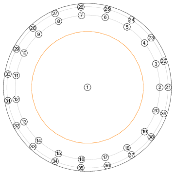
Figure 1: The geometry of the mirror actuators (for 39- and 38- channel version; 38-channel version doesn’t have the central actuator). Diameters of a) the external ring of actuators is 48 mm; b) internal ring of actuators is 43 mm; c) recommended light aperture (shown in orange) is 33 mm.
{/slider} {slider=System setup}
3 Assembling and running of the adaptive optical system
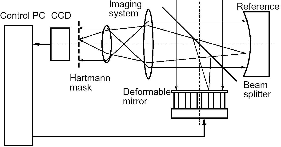
Figure 2: Scheme of typical adaptive optics setup.
Place the mirror and the wavefront sensor into an optical setup. The optical scheme should satisfy the following conditions.
a) The optics should re-image the plane of the mirror to the plane of the Hartmann mask (or microlens array).
b) The scheme should scale the beam in such a way that the working aperture of the mirror (about 35 mm) should be re-imaged to the working area of the Hartmann mask/microlens array (4.5 mm).
c) The optics should allow for calibration. In the general case, it consists of separate measurement of the complete setup aberration with ideal object or a source of ideal wavefront, replacing the one to be tested.
The typical setup for functional feedback loop is shown in the Figure 2.
Connect the wavefront sensor and the deformable mirror; turn on the amplifier units.
Start FrontSurfer. Turn on the preview mode in FrontSurfer and check an image from the Hartmann sensor for both the calibration beam and those reflected from the mirror. It is highly desirable to provide that no spots are missing.
Go to the menu command “Mirror → Set values”. Now you may start to use the mirror by applying different control voltages to the actuators. See FrontSurfer manual for instructions on using of the feedback loop operation mode.
3.1 Practical tips
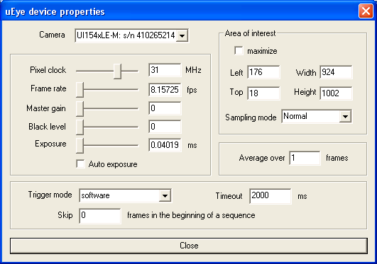
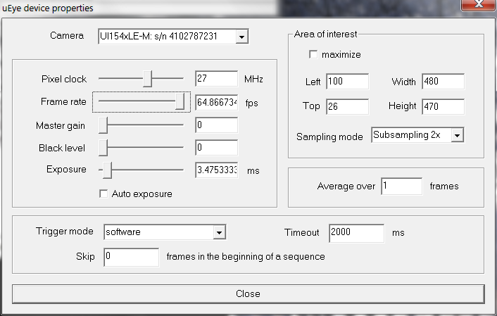
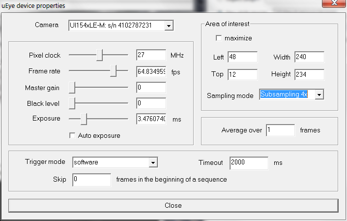
Figure 3: “uEye” plugin properties; settings for “Normal”, “Subsampling x2” and “Subsampling x4” modes (top to bottom).
- Start FrontSurfer. Go to menu “Mirror → Set values” and set value 0 to all actuators. It corresponds to the bias voltage, which produces slightly concave shape on the mirror.
- Make sure that the beam is centered on the deformable mirror, wavefront sensor and other components. You can use the supplied “defocus.exe” or “set_channel.exe 1” command line utilities (supplied on the CD) to facilitate the alignment process.
- Turn on the preview mode in FrontSurfer and check an image from the Hartmannsensor. Adjust the wavefront sensor position for centering.
- Adjust the beam brightness with laser diode power potentiometer and/or polarization filter and the wavefront sensor exposure (use menu “Options ⇒ Camera” and then “Properties” button; see Figure 3) to make the spots good visible, avoiding the saturation.
- Switch on the imaging camera and adjust the exposure to see the focal spot. If needed, adjust the camera position to achieve the best focus.
- In menu “Mirror ⇒ Feedback parameters”, set the parameters according to Figure 4. We recommend setting “Delay” to 100 ms for calibration; it can be reduced to 1 ms for the closed-loop operation.
- If used in a reference mode, take a reference pattern (use menu “File ⇒ Open Reference” or use a shortcut button “2”).
- Go to menu “Mirror ⇒ Calibrate mirror” to calibrate the system. The calibration data can be saved for further use from menu “Mirror ⇒ Save calibration”.
- Check the eigen modes of the system (use menu “Mirror ⇒ Singular values” and double-click on a singular value marker to see the corresponding mode). They should look similar to the modes shown in Fig. ??. Noisy or low-contrast modes indicate an alignment/calibration problem.
- Now you may start closed-loop correction from menu “Mirror ⇒ Start feedback”. During the correction loop, you may compensate for residual static aberration of the system by manually adjusting Zernike terms, in particular, defocus (C[2,0]) and astigmatism (C[2,2] and C[2,-2]). Spot sharpness should be improved.
Please refer to FrontSurfer manual for further information about the feedback loop operation mode.
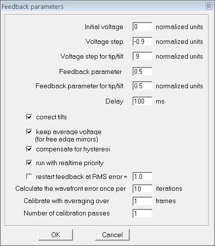
Figure 4: Feedback parameters for calibration of the mirror
{/slider} {slider=Test Results}
4 Mirror testing
{tab= Initial shape of the mirror}
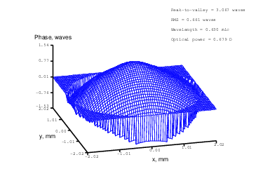
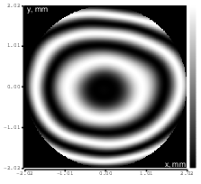
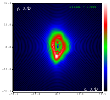
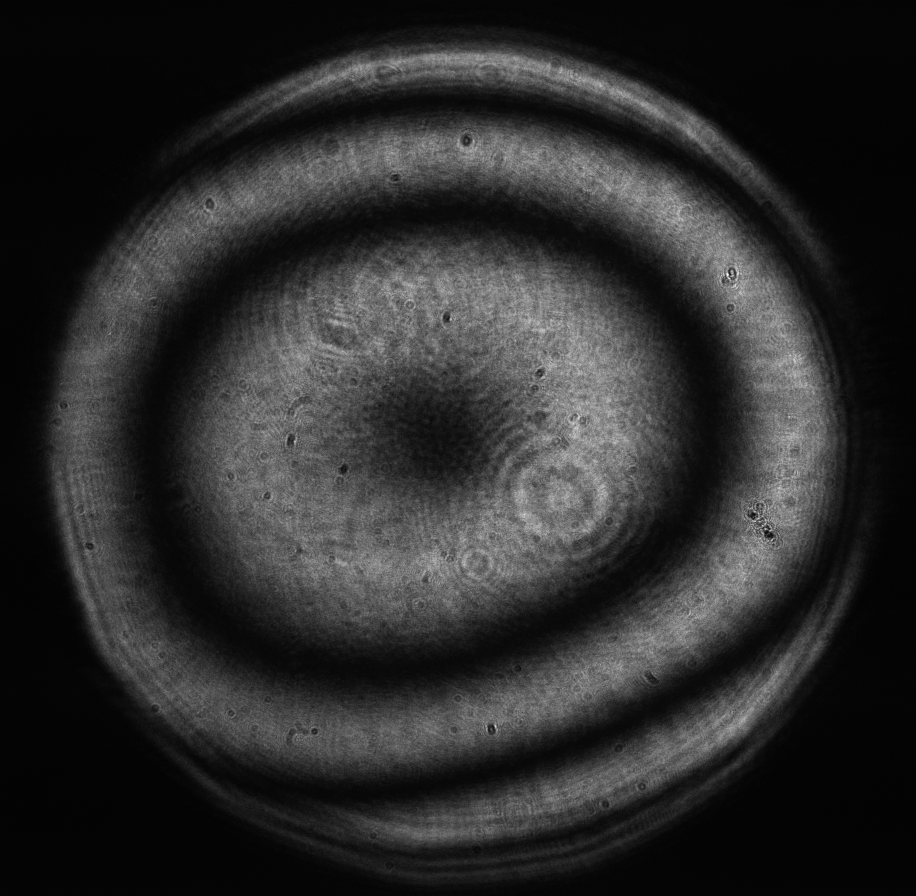
Figure 5: Initial aberration of the system. top: reconstructed wavefront (left) and simulated interferogram (right); simulated far field (left) and registered interferogram (right) .
{tab= Flattened shape of the mirror}
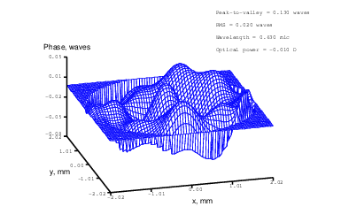
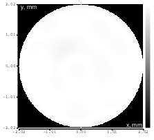
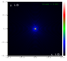
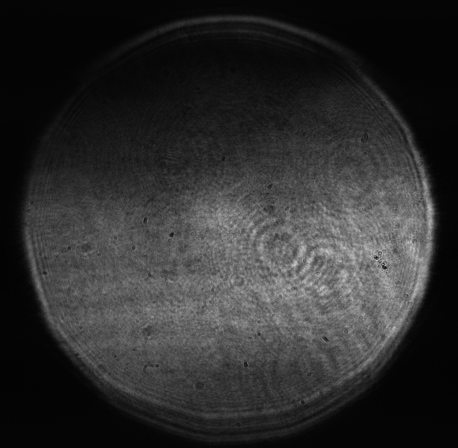
Figure 6: Flattened mirror top: reconstructed wavefront (left) and simulated interferogram (right); simulated far field (left) and registered interferogram (right) .
{tab= Tilt}
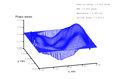
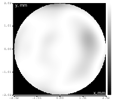
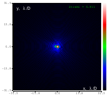
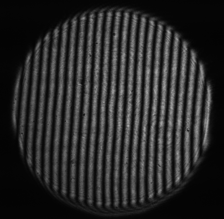
Figure 7: Tilt (Zernike term Z[1,-1]) of amplitude 7.6μm generated. top: reconstructed wavefront (left) and simulated interferogram (right); simulated far field (left) and registered interferogram (right) .
{tab= Defocus}
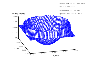
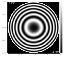
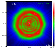
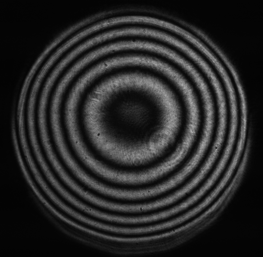
Figure 8: Defocus (Zernike term Z[2,0]) of amplitude 2.2μm generated. top: reconstructed wavefront (left) and simulated interferogram (right); simulated far field (left) and registered interferogram (right) .
{tab= Negative defocus}
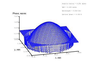
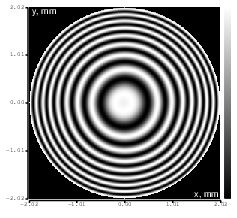
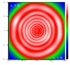
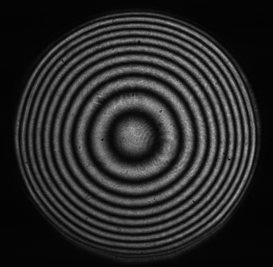
Figure 9: Defocus (Zernike term Z[2,0]) of amplitude -3.2μm generated. top: reconstructed wavefront (left) and simulated interferogram (right); simulated far field (left) and registered interferogram (right) .
{tab= Astigmatism}
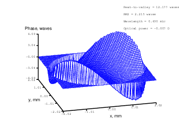
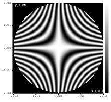
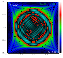
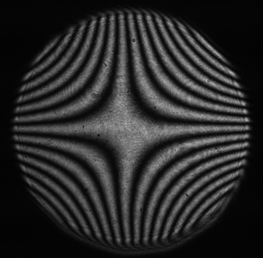
Figure 10: Astigmatism (Zernike term Z[2,2]) of amplitude 4.8μm generated. top: reconstructed wavefront (left) and simulated interferogram (right); simulated far field (left) and registered interferogram (right) .
{tab= Astigamtism}
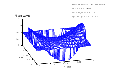

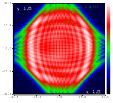
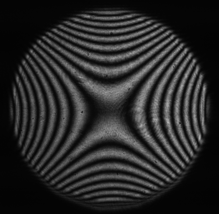
Figure 11: Astigmatism (Zernike term Z[2,-2]) of amplitude -5.4μm generated. top: reconstructed wavefront (left) and simulated interferogram (right); simulated far field (left) and registered interferogram (right) .
{tab= Coma}
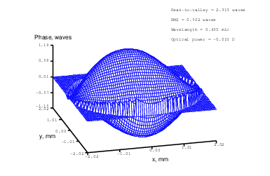
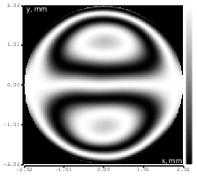
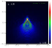
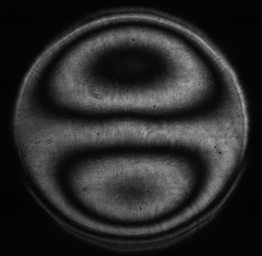
Figure 12: Coma (Zernike term Z[3,1]) of amplitude 1.2μm generated. top: reconstructed wavefront (left) and simulated interferogram (right); simulated far field (left) and registered interferogram (right) .
{tab= Coma}
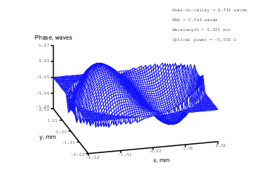
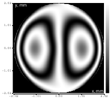
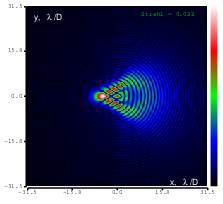
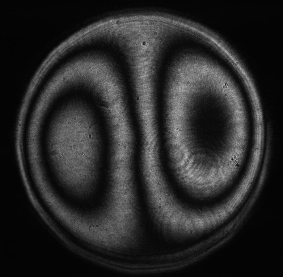
Figure 13: Coma (Zernike term Z[3,-1]) of amplitude 1.3μm generated. top: reconstructed wavefront (left) and simulated interferogram (right); simulated far field (left) and registered interferogram (right) .
{tab= Trefoil}
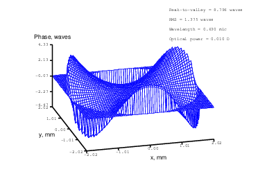
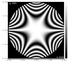
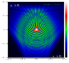
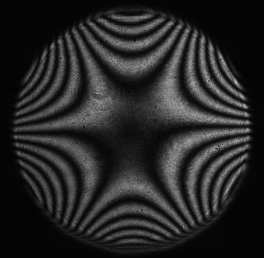
Figure 14: Trefoil (Zernike term Z[3,3]) of amplitude 3.9μm generated. top: reconstructed wavefront (left) and simulated interferogram (right); simulated far field (left) and registered interferogram (right) .
{tab= Trefoil}
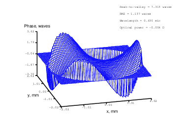
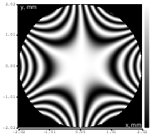
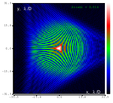
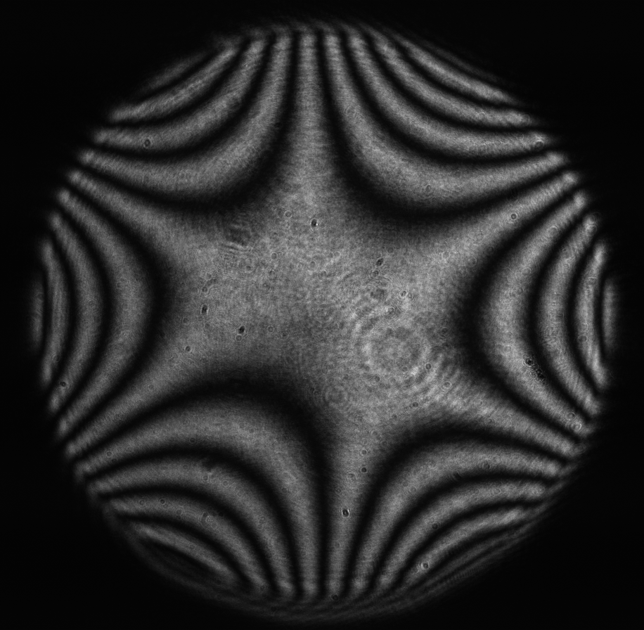
Figure 15: Trefoil (Zernike term Z[3,-3]) of amplitude 3.2μm generated. top: reconstructed wavefront (left) and simulated interferogram (right); simulated far field (left) and registered interferogram (right) .
{tab= Spherical}
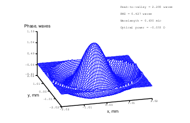
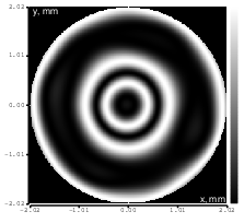

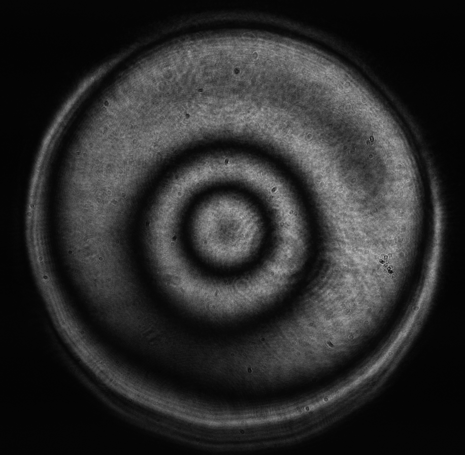
Figure 16: Spherical aberration (Zernike term Z[4,0]) of amplitude 0.7μm generated. top: reconstructed wavefront (left) and simulated interferogram (right); simulated far field (left) and registered interferogram (right) .
{tab= Z[4,2]}
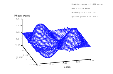
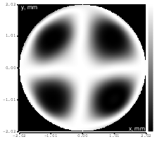
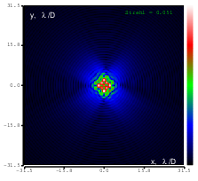
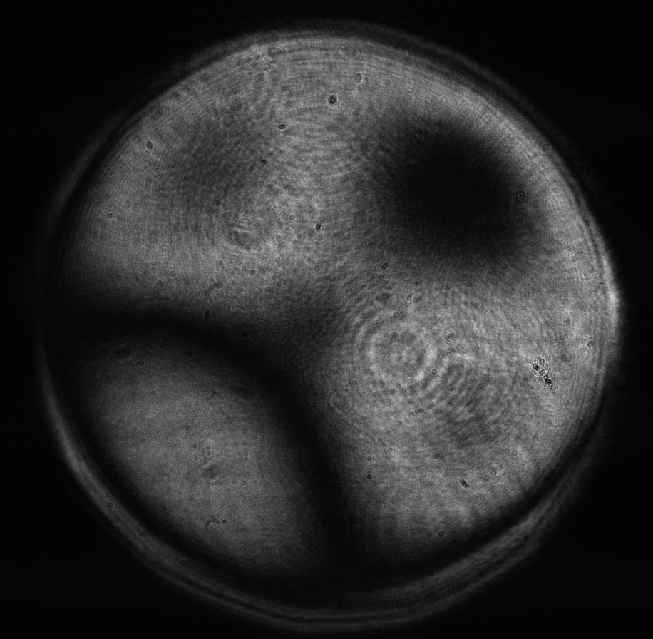
Figure 17: Zernike term Z[4,2] of amplitude 0.6μm generated. top: reconstructed wavefront (left) and simulated interferogram (right); simulated far field (left) and registered interferogram (right) .
{tab= Z[4,-2]}
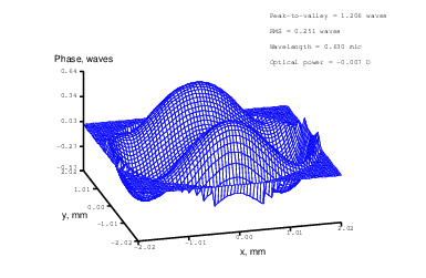
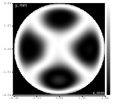
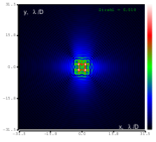
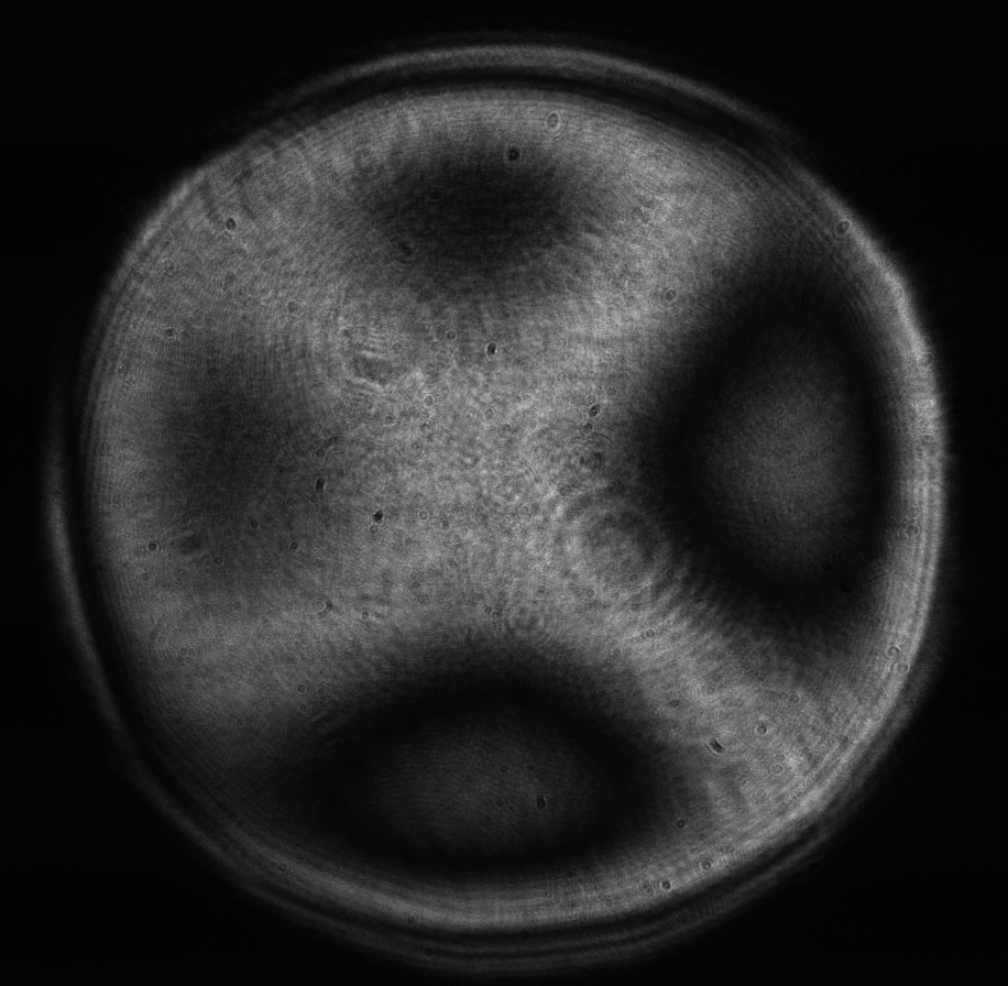
Figure 18: Zernike term Z[4,-2] of amplitude 0.7μm generated. top: reconstructed wavefront (left) and simulated interferogram (right); simulated far field (left) and registered interferogram (right) .
{tab= Z[4,4]}
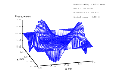
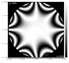
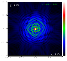
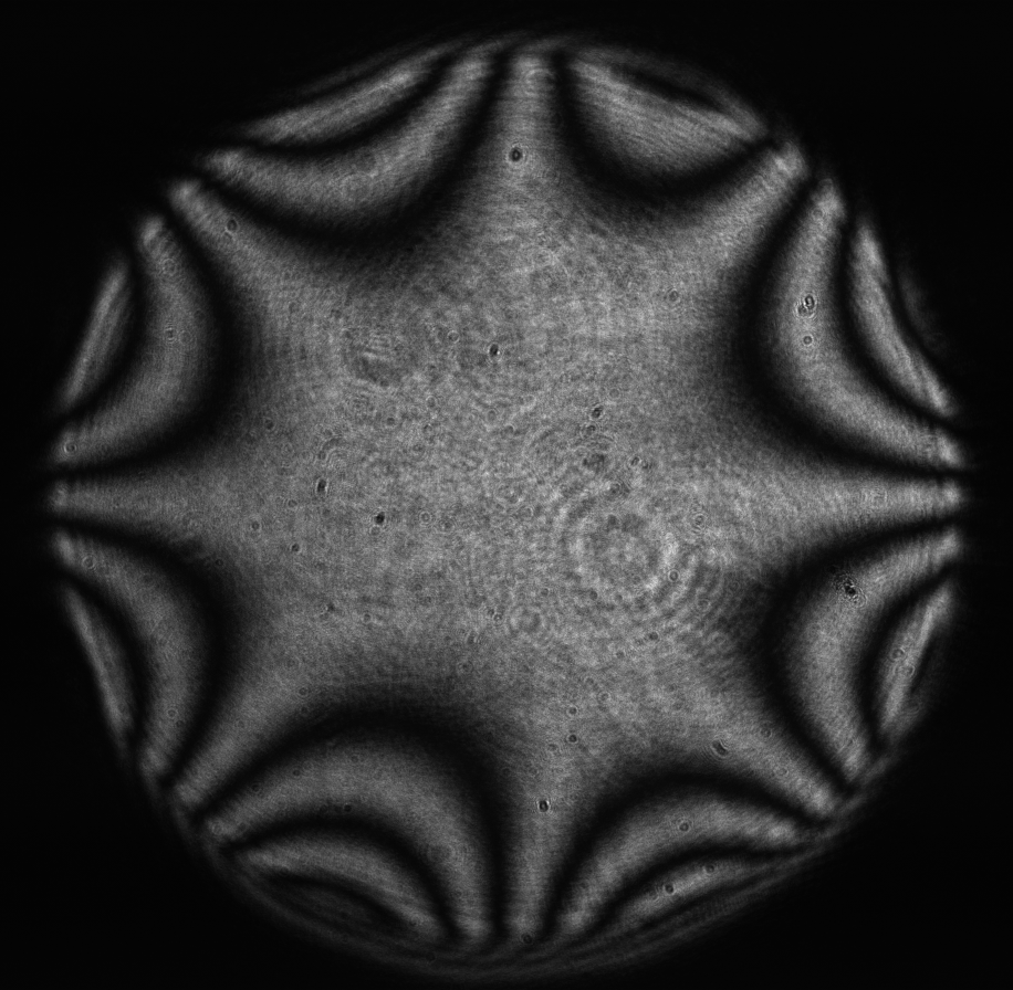
Figure 19: Zernike term Z[4,4] of amplitude 1.9μm generated. top: reconstructed wavefront (left) and simulated interferogram (right); simulated far field (left) and registered interferogram (right) .
{tab= Z[4,-4]}
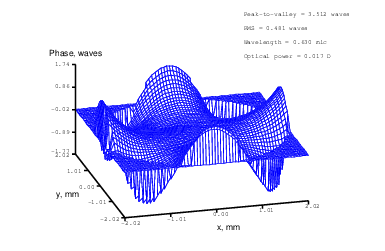
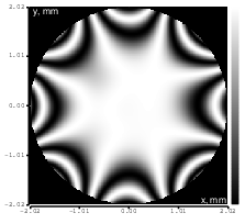
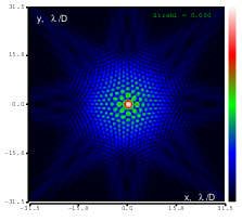
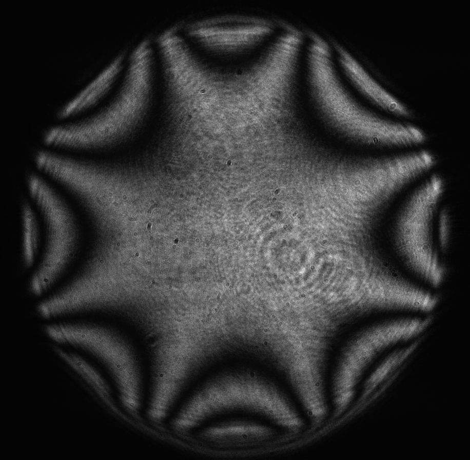
Figure 20: Zernike term Z[4,-4] of amplitude 1.7μm generated. top: reconstructed wavefront (left) and simulated interferogram (right); simulated far field (left) and registered interferogram (right) .
{/tabs}
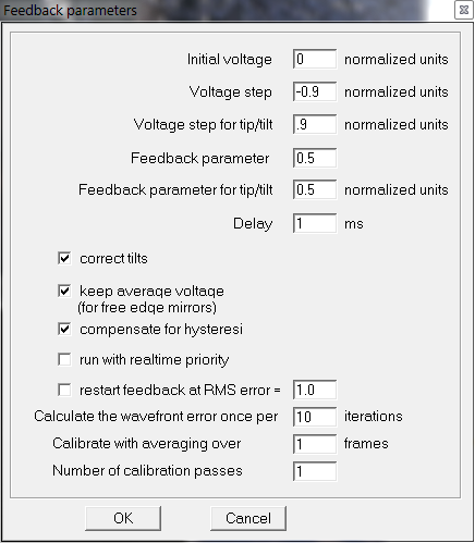
Figure 21: Settings in the “Feedback parameters” dialog box used throughout the tests.
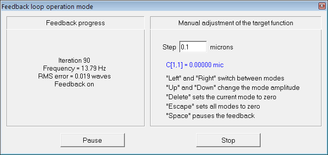
Figure 22: Feedback
A flat mirror was used as a reference. We have used 300:40 mm telescope to conjugate the DM pupil to the WFS plane.
Optimization started from the initial shape of the mirror, which was produced by setting all mirror values to zero; this shape is shown in Figure 5.
In the first test we generated the flat wavefront with respect to the reference mirror. In the following tests we generated various Zernike aberrations with the maximum possible amplitude for which rms error was less than λ∕14 (Maréchal criterion); the results are shown in Figures 8-20. Figure 21 shows the settings of the ”Feedback parameters” dialog box used throughout the tests, and Figure 22 shows the feedback speed achieved during the test (“normal”sub-sampling mode).
{/slider}